MATLAB is a programming platform that has been designed for scientists and engineers alike. Fundamentally, MATLAB is used to analyze data, develop algorithms, and create both models and applications. What separates MATLAB from other programs is the matrix-based language which allows for the natural expression of computational mathematics. The built-in math functions, language, and applications enable a quick exploration of many approaches to a solution.
MATLAB has a wide variety of uses, including machine learning, signal processing, and communications, image and video processing, control systems, tests and measurements, computational finance, and computational biology.
Computer Vision is a field that has become more and more relevant in recent years, a field that can be explored within MATLAB. Computer Vision, as the name suggests, is the computer’s ability to look at a live video or an image and communicate to a person what it is seeing. Researchers who are looking into Computer Vision generally have two goals or approaches in mind.
The first is the biological point of view, where the computer tries to mimic and create models of a human visual system. The second comes from the engineering perspective, where it aims to build autonomous systems that can perform the same tasks as the human model, maybe even to the point where it surpasses the human model.
Computers can ‘see’ the world, but like animals, they see it differently to humans. In basic terms, computers can see things by counting the number of pixels, combined with measuring the shade of the colours to find borders and estimating the spatial relationships between objects. This can all be done within MATLAB, so long as there is a way to produce an image, such as a webcam.
Below is an example of MATLAB being used to develop a program that can count the number of objects within an image. Use the following slideshow to see what the program outputs after certain lines are executed.
Object Detector Code
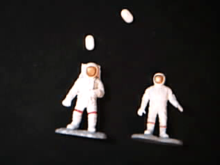
Read in image (Image 1):
color_im = imread('astro.png');
imshow(color_im);
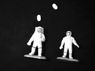
Convert to grayscale (Image 2):
I = rgb2gray(color_im);
imshow(I);
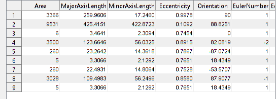
Image Segmentation App:
imageSegmenter(I);Image Region Analyzer App (Image 3):
imageRegionAnalyzer(BW);We have created two scripts for object detection:
- segmentImage.m – converts image to BW
- filterRegions – removes noise from image and gives properties needed from the image
Now call these two functions on a sample image
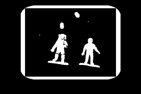
imshow(I);Test the Segment Image Function (Image 4):
BW = segmentImage(I); % segments the image
imshow(BW);
Test the filter regions functions:
properties = filterRegions(BW);
total_count = height(properties)
total_count = 4
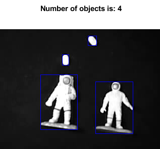
Display results (Image 5):
rgb = insertShape(I,'rectangle',[properties.BoundingBox],'color','blue');
imshow(rgb);
title("Number of objects is: " + total_count);
It is important to understand what the purpose of the functions are, most importantly the segmentImage.m and the filterRegions functions. These are both functions that are applied to a specific image, as the lighting, angle and contrast will be different for different pictures.
The segmentImage.m function is generated based on the brightness of the image, for the specific image the function is shown below:
function [BW,maskedImage] = segmentImage(X)
% Threshold image - adaptive threshold
BW = imbinarize(X, 'adaptive', 'Sensitivity', 0.29, 'ForegroundPolarity', 'bright');

% Create masked image.
maskedImage = X;
maskedImage(~BW) = 0;
end
The filterRegions function is much more important as it requires a human to filter out the unnecessary ‘noise’ that the computer thinks is an object. The effect this has on the image recognition is shown before the results are displayed, where the computer identifies everything as an object. It is only after it is filtered that the 4 objects are identified and highlighted by the program.
function properties = filterRegions(BW_in)

BW_out = BW_in;

% Filter image based on image properties.
BW_out = bwpropfilt(BW_out, 'Area', [100 + eps(100), Inf]);
BW_out = bwpropfilt(BW_out, 'Area', [250, 9531]);
BW_out = bwpropfilt(BW_out, 'MajorAxisLength', [0, 150]);


% Get properties.
properties = regionprops(BW_out, {'Area', 'BoundingBox','Eccentricity', 'EquivDiameter', 'EulerNumber', 'MajorAxisLength', 'MinorAxisLength', 'Orientation', 'Perimeter'});

% Sort the properties.
properties = sortProperties(properties, 'Area');

% Uncomment the following line to return the properties in a table.
properties = struct2table(properties);


function properties = sortProperties(properties, sortField)

% Compute the sort order of the structure based on the sort field.
[~,idx] = sort([properties.(sortField)], 'descend');

% Reorder the entire structure.
properties = properties(idx);
